Exploring spiking neural networks: a comprehensive analysis of mathematical models and applications

Sanaullah 1 * Shamini Koravuna 2 Ulrich Rückert 2 Thorsten Jungeblut 1

• 1 Industrial the Internet of Things, Department of Engineering and Mathematics, Bielefeld University of Applied Sciences and Arts, Bielefeld, Germany
• 2 AG Kognitronik & Sensorik, Technical Faculty, Universität Bielefeld, Bielefeld, Germany

This article presents a comprehensive analysis of spiking neural networks (SNNs) and their mathematical models for simulating the behavior of neurons through the generation of spikes. The study explores various models, including LIF and NLIF, for constructing SNNs and investigates their potential applications in different domains. However, implementation poses several challenges, including identifying the most appropriate model for classification tasks that demand high accuracy and low-performance loss. To address this issue, this research study compares the performance, behavior, and spike generation of multiple SNN models using consistent inputs and neurons. The findings of the study provide valuable insights into the benefits and challenges of SNNs and their models, emphasizing the significance of comparing multiple models to identify the most effective one. Moreover, the study quantifies the number of spiking operations required by each model to process the same inputs and produce equivalent outputs, enabling a thorough assessment of computational efficiency. The findings provide valuable insights into the benefits and limitations of SNNs and their models. The research underscores the significance of comparing different models to make informed decisions in practical applications. Additionally, the results reveal essential variations in biological plausibility and computational efficiency among the models, further emphasizing the importance of selecting the most suitable model for a given task. Overall, this study contributes to a deeper understanding of SNNs and offers practical guidelines for using their potential in real-world scenarios.

1. Introduction

Artificial General Intelligence (AGI) strives to emulate human-like intelligence in machines, encompassing the ability to perform a wide array of cognitive tasks with high precision, robustness, and efficiency (Goertzel, 2014). As the pursuit of AGI continues, researchers have been exploring innovative brain-inspired approaches to achieve these ambitious goals. In this context, several representative studies have emerged, showcasing promising advancements in brain-inspired intelligence and their potential to outperform state-of-the-art artificial intelligence systems (Mehonic et al., 2020). These groundbreaking works have garnered significant attention in the field, as they lay the foundation for high-level intelligence, accuracy, robustness, and energy efficiency. Therefore, some representative studies exemplify the state-of-the-art efforts in brain-inspired artificial intelligence, offering valuable and inspiring new directions for achieving AGI with unprecedented capabilities (Stimberg et al., 2019; Sanaullah et al., 2022a,b). By combining the principles of neuroscience with advanced machine learning techniques, such as SNNs, these novel approaches hold the potential to revolutionize the field and drive AGI toward realization.

SNNs are a type of neural network model that has gained considerable attention in recent years due to their ability to simulate the behavior of biological neurons in the brain (Ghosh-Dastidar and Adeli, 2009b; Sanaullah et al., 2023a). SNNs are characterized by their discrete time steps, where the neurons generate spikes when the input reaches a certain threshold (Tavanaei et al., 2019; Sanaullah et al., 2020). This is similar to how biological neurons work, where they communicate with each other through the generation of action potentials or spikes (Tavanaei et al., 2019).

To build an SNN, a mathematical model of the spiking behavior of neurons is required. Several models have been developed, each with its own advantages and limitations. One of the most commonly used models is the leaky integrate-and-fire (LIF) model (Brunel and Van Rossum, 2007), which models the behavior of neurons as a leaky capacitor that charges and discharges over time. The Adaptive Exponential (AdEx) model (Gerstner and Brette, 2009), is another popular model that includes an exponential term to account for the adaptation of neuron firing rates over time. The Non-linear Integrate-and-Fire (NLIF) model (Jolivet et al., 2004), is a more complex model that includes non-linearity in the integration process. Other SNN models include the Integrate-and-Fire with Spike Frequency Adaptation (IF − SFA) model (Gigante et al., 2007), which incorporates a feedback mechanism that adjusts the neuron's firing rate based on its recent activity, the Theta Neuron model (McKennoch et al., 2009), which models the theta rhythm observed in the brain, the Hodgkin-Huxley (HH) model (Häusser, 2000), which is a biophysical model that includes multiple ion channels to capture the complex behavior of neurons, and the Quadratic-Integrate-and-Fire (QIF) model (Brunel and Latham, 2003), which is a more general model that allows for different types of threshold functions. Another widely used model in SNNs is the Izhikevich model (Izhikevich, 2004, 2007), which offers a balance between computational efficiency and biological plausibility. This model introduces a two-variable system that captures the dynamics of the neuron's membrane potential and recovery variable. The IZH model can replicate a wide range of spiking patterns observed in real neurons, making it suitable for various computational tasks. Additionally, the Spike Response Model (SRM; Gerstner, 2008), is another significant model in SNNs. The SRM focuses on capturing the post-spike response characteristics of neurons, which include the refractory period and the shape of the post-spike potential. By considering these response dynamics, the SRM provides a more detailed description of neuron behavior and enables the modeling of temporal effects in neural computations. Therefore, each of these models offers its own set of advantages and limitations, providing researchers and engineers with a diverse toolbox to simulate and understand the behavior of spiking neurons.

In addition to the challenges of selecting the most suitable SNN model, another challenge associated with SNNs is the need for specialized simulators to simulate the spiking behavior of neurons. One popular simulator used for SNNs is the Neural Engineering Framework (NEF; Stewart, 2012; Sanaullah et al., 2023b), which is a mathematical framework for designing and implementing neural models that are based on the principles of neuroscience. Despite the potential benefits of SNNs, there are still several challenges associated with their implementation. One of the most significant challenges is choosing the most appropriate SNN model for a given task (Stimberg et al., 2019; Sanaullah et al., 2022a,b).

This is particularly important for classification tasks, where accuracy and performance loss are critical. Another challenge is the computational complexity of simulating SNNs, which can require significant computational resources (Ayan et al., 2020). Therefore, choosing the appropriate SNN model and addressing the computational complexity associated with their simulation remain significant challenges that need to be addressed to realize their full potential.

In order to address this issue, a study was conducted to compare the performance, behavior, and spikes generation methodology of different SNN models using the same number of inputs and neurons. The challenge of determining the most suitable model was addressed by comparing the performance of different models, and the results were analyzed to determine the most effective one. Additionally, the study also compared the biological plausibility of the different neuron models used in the SNNs. The biological plausibility of a neuron model is an important factor to consider since it determines how well the model simulates the behavior of actual biological neurons. The study also compared the number of spiking operations required by each model to simulate the behavior of the same set of neurons. The results showed that the LIF models required the least number of spiking operations, while the HH model required the most. These findings could aid in selecting the most appropriate SNN model based on the specific requirements of the task, such as accuracy, biological plausibility, and computational efficiency. Overall, this study sheds light on the challenges and potential benefits of SNNs and their models. It highlights the importance of comparing different models to determine the most suitable and provides valuable insights for researchers and practitioners working in this area.

2. Background

Artificial neural networks are computational models inspired by the structure and function of the brain, aimed at replicating and understanding human abilities (Bishop, 1995). Unlike traditional artificial neural networks, which use continuous activation functions to transmit information, SNNs use a “spike train” representation, where the output of each neuron is a series of discrete spikes (Ghosh-Dastidar and Adeli, 2009a,c). This allows SNNs to model the precise timing and sequencing of neural activity, making them well-suited for tasks that require the processing of temporal patterns and spatiotemporal information (Zhang and Li, 2019). Therefore, these networks have found widespread use in machine learning tasks such as function approximation and pattern recognition (Le, 2013; Krizhevsky et al., 2017).

As AGI research progresses, these works will continue to serve as critical reference points for developing more efficient, intelligent, and adaptive artificial intelligence systems with real-world applications in diverse domains (Graves et al., 2008; Sanaullah et al., 2023a). Therefore, some critical research works have significantly contributed to the development of AGI through brain-inspired paradigms, highlighting their key contributions and implications for the future of artificial intelligence.

• Robust Spike-Based Continual Meta-Learning Improved by Restricted Minimum Error Entropy Criterion by Yang et al. (2022c): This pioneering study introduces a novel spike-based framework that uses entropy theory for online meta-learning in a recurrent SNN. MeMEE improves spike-based meta-learning performance, shown through tasks like autonomous navigation and working memory tests. It emphasizes the integration of advanced information theory in machine learning, offering new perspectives for spike-based neuromorphic systems.

• Heterogeneous Ensemble-based Spike-driven Few-shot Online Learning by Yang et al. (2022b): a novel spike-based framework employing entropy theory for few-shot learning in recurrent SNNs. The HESFOL model significantly enhances the accuracy and robustness of few-shot learning tasks in spiking patterns and the Omniglot dataset, as well as in few-shot motor control tasks. Our study emphasizes the application of modern entropy-based machine learning in state-of-the-art spike-driven learning algorithms.

• SAM: A Unified Self-Adaptive Multicompartmental Spiking Neuron Model for Learning with Working Memory introduced by Yang et al. (2022a): a self-adaptive spiking neuron model integrating spike-based learning with working memory. SAM shows efficient and robust performance across tasks like supervised learning, pattern classification, and meta-learning, making it valuable for neuromorphic computing in robotics and edge applications. It also offers insights into the biological mechanisms of working memory.

• Neuromorphic Context-dependent Learning Framework with Fault-tolerant Spike Routing (Yang et al., 2021a): This study introduces a scalable neuromorphic fault-tolerant hardware framework for event-based SNNs. It successfully learns context-dependent associations despite possible hardware faults, enhancing network throughput by 0.9–16.1%. The proposed system enables real-time learning, decision-making, and exploration of neuronal mechanisms in neuromorphic networks.

Furthermore, SNNs use mathematical models to simulate the behavior of biological neurons. These models capture the complex behavior of neurons, including the propagation and integration of electrical signals, as well as the refractory period during which a neuron cannot fire a new spike (Tavanaei et al., 2019; Wang et al., 2020). At a high level, SNNs are models of biological neural networks that simulate the behavior of neurons in the brain using mathematical equations. These equations capture the electrical and chemical activity that occurs within neurons and between them. The basic building block of an SNN is the spiking neuron, which models the behavior of a biological neuron that fires an action potential, or spike when it receives enough input. SNNs also use mathematical models to describe the connectivity between neurons. For example, a common model is the synapse model, which describes the strength and dynamics of the connections between neurons based on neurotransmitter release and reuptake (Deco et al., 2008). Overall, the mathematical models used in SNNs allow us to simulate the complex behavior of biological neural networks and understand how they process information. These models can also be used to develop new algorithms for machine learning and artificial intelligence, which are inspired by the way the brain processes information.

3. Results and discussion

Neuromorphic computing is a novel computing paradigm known for its low power consumption and high-speed response. Several notable research works in the field are worth mentioning. For instance, the “Smart Traffic Navigation System for Fault-Tolerant Edge Computing of Internet of Vehicles in Intelligent Transportation Gateway (Yang et al., 2023)” focuses on developing a fault-tolerant edge computing system for the Internet of Vehicle applications in intelligent transportation. “CerebelluMorphic” is a large-scale neuromorphic model and architecture designed for supervised motor learning (Yang et al., 2021c). Lastly, “BiCoSS” aims to create a large-scale cognitive brain with a multi-granular neuromorphic architecture (Yang et al., 2021b). These innovative works contribute to the advancement of neuromorphic computing and demonstrate its potential in various applications, from fault-tolerant edge computing to large-scale motor learning and cognition systems.

SNN models are typically built using mathematical equations that describe the behavior of spiking neurons. These equations take into account various factors such as the input current, membrane potential, and membrane time constant, to simulate the behavior of biological neurons. Each SNN model has its own set of equations that determine its behavior. In the study mentioned, different SNN models have been investigated. These include namely LIF, NLIF, AdEx, IF − SFA, ThNeuron, HH, QIF, IZH, and SRM models. Each of these models is implemented using the update method, which takes an input current and a time step and returns whether a spike has occurred or not. The update method uses the equations that describe the behavior of the spiking neurons to calculate the membrane potential of each neuron at each time step. If the membrane potential exceeds a certain threshold, a spike is generated and propagated to the next neurons. By investigating different SNN models, researchers can gain a better understanding of how the brain processes information and how to design more efficient and accurate artificial neural networks. SNN models have potential applications in various fields, including robotics, computer vision, and natural language processing.

Therefore, this study provides a comprehensive analysis of SNNs and their mathematical models and contributes to progress in the research discipline by addressing the challenges in implementing SNNs for classification tasks that demand high accuracy and low-performance loss using a simulational environment. The study compares the performance, behavior, and spike generation of different SNN models using the same inputs and neurons, providing valuable insights into the benefits and challenges of SNNs and their models. The study also quantifies the number of spiking operations required by each model to process the same inputs and output the same results, providing a comparative analysis of the computational efficiency of the models.

3.1. Types of SNN models

We initialize the instance variables for each model and generate random weights for each neuron. One of the simplest SNN models is the LIF model, which is described by Equation 1:

where τ_m is the time constant, V(t) is the membrane potential of the neuron at time t, and I(t) is the input current at time t. The membrane potential is updated based on the Equation 2:

If membrane potential reaches the threshold potential V_th, the neuron fires a spike and the membrane potential is reset to the resting potential V_reset, which is described in Equation 3:

A variation of the LIF model is the Non-Linear Integrate-and-Fire (NLIF) model, which takes into account the non-linear relationship between the membrane potential and the input current. The NLIF model is described by Equation 4:

where V is the membrane potential, I is the input current, τ is the membrane time constant, and d V d t represents the change in the membrane potential over time. The membrane potential is updated based on the Equation 5:

where V_reset is the resting potential, α and β are scaling factors, and V_th is the threshold potential. The membrane potential is multiplied by β if it is below the threshold, which models the leakage of current from the neuron over time. If the membrane potential reaches the threshold potential, the neuron fires a spike and the membrane potential is reset to the resting potential plus a scaled depolarization of the membrane potential (as described by Equation 6):

Another SNN model is the AdEX model, which captures the dynamic behavior of spiking neurons more accurately than the LIF or NLIF models. The AdEx model is described by Equation 7:

where V is the membrane potential of the neuron, I is the input current, τ_m is the membrane time constant, V_rheo is the rheobase potential, Δ_T is the slope factor, and V_spike is the threshold potential at which the neuron fires an action potential. If V exceeds V_spike, a spike is generated and V is reset to V_reset.

The IF − SFA model is another SNN model that incorporates the adaptation of the firing rate of neurons in response to input stimuli. The model is based on the LIF model with an additional adaptation current, which modifies the membrane potential and firing rate of the neuron over time. The IF − SFA model is described by Equation 8:

where τ_m is the time constant, V(t) is the membrane potential of the neuron at time t, I(t) is the input current at time t, and w(t) is the adaptation current. The membrane potential is updated based on the following equations:

where Δt is the time step, τ_w is the time constant for the adaptation current, A is the adaptation strength, and V_rest is the resting potential of the neuron. The adaptation current w(t) is computed based on the difference between the membrane potential and the resting potential, and is added to the input current in Equation 8. The membrane potential is updated based on Equation 10, where the adaptation current is subtracted from the input current.

If the membrane potential reaches the threshold potential V_th, the neuron fires a spike and the membrane potential is reset to the resting potential V_rest. The adaptation current is also updated according to Equation 11:

where b is a constant that represents the increase in the adaptation current after a spike is generated. The increase in the adaptation current leads to a decrease in the firing rate of the neuron over time, allowing the neuron to adapt to the input stimulus.

The ThetaNeuron model is a more complex model that incorporates the influence of a sinusoidal waveform, in addition to the input current and membrane potential. The ThetaNeuron model is described by Equation 12:

where V is the membrane potential, I_syn is the synaptic input current, I_ext is the external input current, I_theta is the sinusoidal input current, and τ_m is the membrane time constant. The sinusoidal input current is described by Equation 13:

where I_thetamax is the amplitude of the sinusoidal input current, f_theta is the frequency of the theta rhythm, t is the time, and ϕ is the phase of the theta rhythm. The membrane potential is updated based on the Equation 14:

where V_reset is the resting potential and V_th is the threshold potential. If the membrane potential reaches the threshold potential, the neuron fires a spike and the membrane potential is reset to the resting potential.

Furthermore, the ThetaNeural model incorporates a sinusoidal input current in addition to the synaptic and external input currents to update the membrane potential based on Equation 12. If the membrane potential reaches the threshold potential, the neuron fires a spike and the membrane potential is reset to the resting potential as described by the Equation 14. The HH and QIF models are fundamentally different from the LIF, NLIF, and AdEx models because they do not use differential equations to model the behavior of neurons. The HH model is a biophysical model that simulates the behavior of ion channels and currents in the neuron membrane. It is described by a system of differential equations that represent the time-dependent behavior of ion channels. The QIF model, on the other hand, is a simplified model that assumes that the neuron fires an action potential whenever its membrane potential crosses a threshold. The QIF model is described by Equation 15:

where V_i is the membrane potential of the neuron at time step i, C is the capacitance of the neuron, g_syn is the conductance of synaptic input, V_syn is the reversal potential of the synaptic input, I_ext is the external current input, and I_noise is the random noise input.

Additionally, the Izhikevich (IZH) model captures the dynamics of real neurons while being computationally efficient. It is described by a set of ordinary differential equations that govern the behavior of the neuron. The model consists of two main variables: the membrane potential, denoted by v(t), and a recovery variable, denoted by u(t). The IZH model is defined by the following equations,

where a, b, and I are parameters that determine the behavior of the neuron. The parameter I represents the input current to the neuron, which can be thought of as the summation of all the incoming currents from other neurons or external sources. The terms 0.04v 2 + 5v + 140 − u and a(bv − u) describe the dynamics of the membrane potential and the recovery variable, respectively. So, the update process of the implemented IZH model involves integrating these equations over time using numerical integration methods, such as Euler's method:

If the membrane potential v(t) exceeds a certain threshold, typically set to 30.0, the neuron is considered to have fired a spike. In that case, the membrane potential is reset to a specific value c, and the recovery variable is incremented by a fixed value d. This reset and increment simulate the after-spike behavior of the neuron. Hence, the update equations after a spike are:

Therefore, the IZH model provides a computationally efficient yet biologically inspired representation of spiking neuron dynamics. By adjusting the parameters a, b, c, and d, different spiking patterns can be replicated, allowing for the modeling of a wide range of neuron behaviors.

In the SRM, each neuron has two variables: the membrane potential, denoted as V_init, and the synaptic variables, denoted as s(t) and r(t). The membrane potential represents the electrical potential across the neuron's membrane, while the synaptic variables capture the post-synaptic response to incoming spikes. It is described by the equations:

where τ_s and τ_r are the time constants for the synaptic and refractory dynamics, respectively. s and r are the synaptic variables, which decay exponentially over time. The input current represents the external input to the neuron, and ∑ i w i s i represents the weighted sum of the incoming spikes from other neurons, where w_i is the weight associated with each connection and s_i is the corresponding synaptic variable of the pre-synaptic neuron. Therefore, the update process of the implemented SRM model involves integrating these equations over time using numerical integration methods:

Additionally, the SRM model includes a threshold potential V_th and a reset potential V_reset. If the membrane potential reaches or exceeds the threshold V_th, the neuron fires a spike, and the membrane potential is reset to V_reset. The synaptic variables s and r are also incremented by 1.0 to represent the post-synaptic response to the spike.

However, it is possible to combine different models in a single network, as long as the models are compatible with each other and can be integrated seamlessly. For example, the HH model can be used to model the behavior of individual neurons in a network, while the QIF model can be used to model the behavior of the network as a whole. However, it is important to note that the HH and QIF models are much more complex and computationally intensive than the simpler SNN models and may not be suitable for all applications (Ma and Wu, 2007).

3.2. Dataset

Datasets play a crucial role in the development and evaluation of machine learning models, including spiking neural networks. They provide the necessary input for the models to learn and make predictions, and the quality and suitability of the dataset can significantly impact the model's performance. There are various types of datasets available for machine learning, including benchmark datasets, real-world datasets, and synthetic datasets. Each type of dataset has its advantages and disadvantages, and the choice of dataset depends on the task at hand and the goals of the study. The MNIST dataset and other benchmark datasets are commonly used for evaluating machine learning models, including spiking neural networks. However, these datasets are limited in terms of their complexity and do not necessarily reflect the challenges of real-world problems. In contrast, synthetic datasets can be tailored to specific tasks and can provide a more controlled environment for comparing different models. The synthetic dataset used in this study was designed to have two classes that are easily separable by a linear classifier, which allows for a straightforward evaluation of the performance of different models. Additionally, the synthetic dataset is more transparent in terms of the underlying data generation process, which can help in identifying the strengths and weaknesses of different models. For example, the MNIST dataset is a well-known benchmark dataset for image classification and the input images are preprocessed and normalized, the performance of each model is expected to be similar, due to the same parameters (tau, v_reset, v_th, alpha, n_neurons, and dt), and the same number of neurons (n_neurons) has been used for almost every model. Therefore, using a synthetic dataset can be a useful tool for comparing and evaluating different spiking neural network models, especially for tasks where real-world datasets are not readily available or do not provide enough complexity.

A synthetic dataset used for this study was generated using the following approach; Let n_samples = 1, 000, x 1 ~ N ( 0 , 1 ) , x 2 ~ N ( 3 , 1 ) , X = [ x 1 x 2 ] , y = [ 0 n s a m p l e s 1 n s a m p l e s ] , where 0_nsamples and 1_nsamples are the vectors of length n_samples filled with zeros and ones, respectively. To shuffle the dataset, let i n d i c e s = [ 0 1 ⋯ 2 n s a m p l e s - 1 ] , and apply a random permutation to indices. Then, let X and y be the arrays obtained by indexing X and y with the shuffled indices.

For example, the dataset contains a total of n_samples = 1, 000 samples, and two features, x₁ and x₂, were generated for each sample using normal distributions. Specifically, x₁ was sampled from a normal distribution with a mean of 0 and a standard deviation of 1, denoted as N ( 0 , 1 ) . On the other hand, x₂ was sampled from a normal distribution with a mean of 3 and a standard deviation of 1, denoted as N ( 3 , 1 ) . The feature matrix for all samples is denoted as X and is represented as follows:

The corresponding labels for the samples were created to form a binary classification problem. The label vector y has a length of 2n_samples, containing n_samples zeros followed by n_samples ones. In mathematical notation:

Here, 0_nsamples represents a vector of length n_samples filled with zeros, and 1_nsamples represents a vector of length n_samples filled with ones. To randomize the dataset, a set of indices, denoted as indices, is created as follows:

This array contains consecutive integers from 0 to 2n_samples−1. Next, a random permutation is applied to the indices array to shuffle the dataset randomly. Finally, the feature matrix X and the label vector y are updated based on the shuffled indices. The elements of X and y are rearranged according to the new order provided by the shuffled indices. As a result of this process, the synthetic dataset with 1,000 samples, each having two features (x₁ and x₂) and corresponding binary labels. This dataset can be used to train and evaluate machine learning models for binary classification tasks.

3.3. Comparison

In this study, the performance of the different SNN neural models was explored using classification accuracy and performance loss as the performance metrics, where classification accuracy measures the percentage of correctly classified samples or data points by a model. Therefore, we used classification accuracy to evaluate how accurately each SNN model classified the input data based on the comparison of predicted spikes with the true labels. The accuracy is calculated as the mean of the element-wise equality comparison and then multiplied by 100 to obtain a percentage value. A higher accuracy indicates a better-performing model in terms of its ability to correctly classify the input patterns. Performance loss, on the other hand, quantifies the deviation or error of the model's predictions from the ground truth or desired output. It provides an indication of the model's ability to accurately represent the input data. In this study, the performance loss is calculated as the error rate, which demonstrates the percentage of misclassified samples. A lower error rate indicates a better-performing model with less deviation from the desired output. It is important to note that the specific definitions and measurements for classification accuracy and performance loss may vary depending on the context and objectives of the study. In our case, these metrics were chosen as they are commonly used in evaluating the performance of classification tasks and provide a straightforward assessment of the SNN models' capabilities.

It is important to note that, the proposed approach of this study does not implement a typical neural network with layers, connectivity, and learning mechanisms. Instead, it presents a collection of different single-neuron models and trains each model individually to classify a synthetic dataset. Each of the defined models (e.g., LIF, NLIF, AdEx, HH, etc.) represents a single-neuron model. These models are not interconnected in a multi-layer network, and there is no learning mechanism such as backpropagation or gradient descent. Therefore, using a single-neuron model have several benefits that make them useful for certain applications and provide clear comparisons.

• Simplicity: Single-neuron models are relatively simple compared to complex multi-layer neural networks. They provide a clear and intuitive understanding of how individual neurons respond to input stimuli and how their dynamics influence their behavior.

• Insight into individual neuron behavior: Each model focuses on a single neuron type and highlights specific properties and behaviors unique to that neuron. This allows researchers to study and compare the characteristics of different neurons in isolation.

• Interpretability: Due to their simplicity, single-neuron models are more interpretable. It is easier to analyze and understand the role of individual model parameters on the neuron's behavior.

• Benchmarking: Single-neuron models can serve as benchmarks for evaluating more complex neural network models. They provide a baseline to compare the performance of more sophisticated models in certain tasks, especially when the task can be effectively handled by a single neuron.

• Model selection: When faced with various neuron models, single-neuron simulations can help select the most suitable model for specific applications. Comparing the responses of different models to various inputs can aid in choosing the one that best captures the desired neuron behavior.

• Biological plausibility: Some of the single-neuron models, such as the Hodgkin-Huxley model, are biologically inspired and attempt to replicate the behavior of real biological neurons. These models help researchers explore and understand the mechanisms underlying neural dynamics.

• Fast simulations: Since single-neuron models have fewer parameters and computations compared to deep neural networks, simulations can be faster and computationally less demanding. This advantage is especially useful when exploring a wide range of parameters or conducting large-scale simulations.

Therefore, this study demonstrates how to simulate and evaluate the spike responses of different single-neuron models in response to a synthetic dataset. It does not implement a traditional neural network with layers and learning mechanisms. Figure 1 shows the accuracy and error rates of each neural model, allowing for a clear comparison of their performance. Among the models, the AdEX model demonstrated the highest accuracy, achieving an accuracy of 90.05% with an error rate of 0.10%. On the other hand, the HH model exhibited the lowest accuracy with error rates of 0.50 and 49.55% respectively, and the SRM model reveal the second lowest accuracy of 49.95% with an error rate of 0.50%. The Izhikevich model obtained an accuracy of 50.05% with an error rate of 0.50%. The simplest neural model, LIF achieved an accuracy of 71.20% with an error rate of 0.32% and the NLIF model achieved an accuracy of 66.55% with an error rate of 0.35%. However, the IF − SFA model also achieved an accuracy of 84.30% with an error rate of 0.14% and the QIF model achieved an accuracy of 70.70% with an error rate of 0.27%. Lastly, the ThetaNeuron model achieved an accuracy of 58.55% with an error rate of 0.42%. Overall, the AdEX model showed the highest accuracy, while the HH, IZH, and SRM models had the lowest accuracy. These accuracy and error rate values provide a quantitative assessment of the performance of each SNN model, allowing for a clear understanding of their relative capabilities in accurately classifying the input spiking patterns.

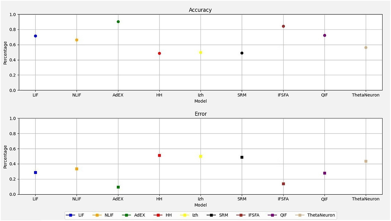
Figure 1. Comparison of accuracy and error rates for different neuron models.

In addition to the accuracy and error rates, we wanted to understand how well each SNN model performed compared to the others. To do this, we used a metric called “performance loss.” Performance loss measures how much a particular SNN model's accuracy deviates from the accuracy of the best model on the dataset. In Table 1, you can see the performance loss of each model relative to the best model. Let's take the LIF model as the reference. The LIF model displayed a performance loss of –45.63% when compared to the ThetaNeuron model, indicating it performed 45.63% worse than the latter. In contrast, the LIF model had a performance loss of –9.36% relative to NLIF, meaning it performed 9.36% worse than NLIF. However, when comparing LIF to AdEx, it showed a performance loss of 20.08%, suggesting that it performed 20.08% better than AdEx.

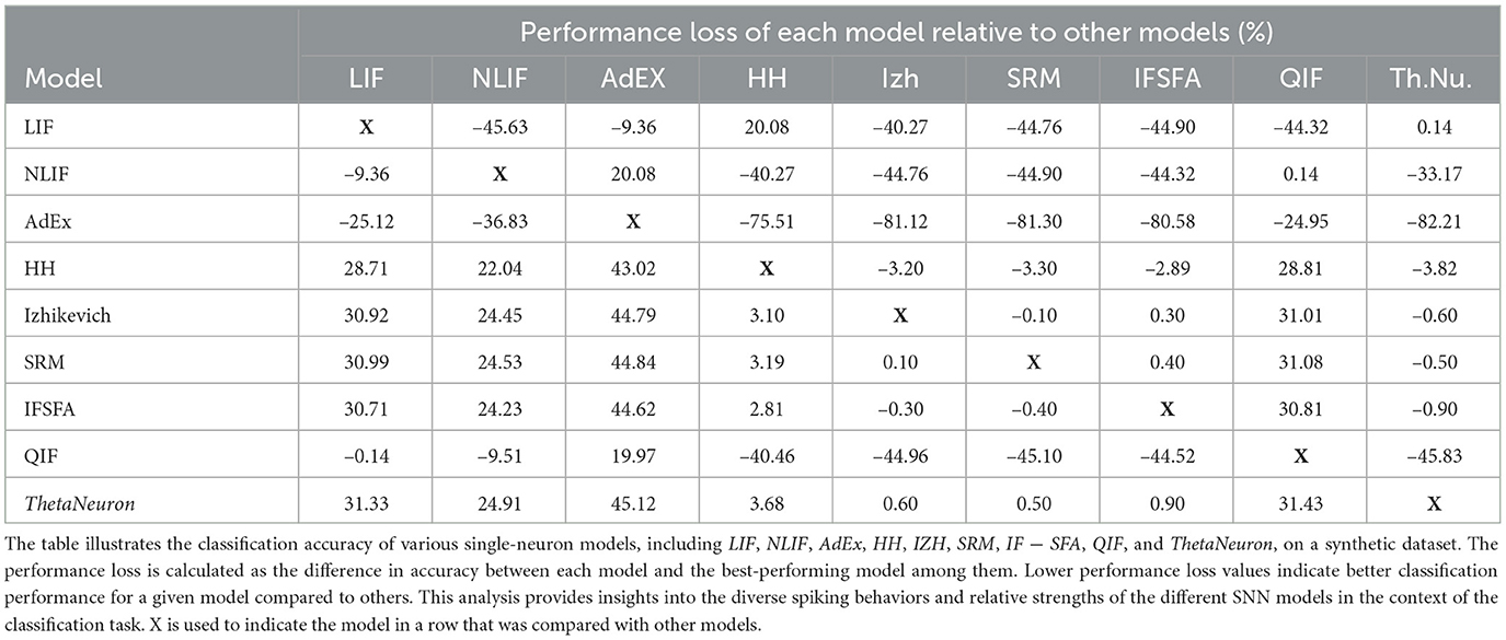
Table 1. Performance loss of different SNN models.

Similarly, the HH model exhibited a performance loss of –40.27% compared to LIF, indicating it performed 40.27% worse than LIF. The Izhikevich model had a performance loss of –44.76% relative to LIF, while the SRM model and the IF − SFA model had performance losses of –44.90 and –44.32% respectively, both compared to LIF. However, when comparing LIF to QIF, the performance loss was only 0.14%, suggesting that their performance was quite similar. Moving on to NLIF, it displayed a performance loss of –33.17% relative to ThetaNeuron, implying it performed 33.17% worse than ThetaNeuron. The performance loss of NLIF compared to HH and Izhikevich was –40.27 and –44.76% respectively, indicating its worse performance in both cases. Similarly, NLIF had a performance loss of –44.90 and –44.32% when compared to SRM and IF − SFA respectively. However, similar to LIF, NLIF showed a negligible performance loss of 0.14% when compared to QIF.

Lastly, let's consider AdEx, which served as the reference model. It displayed a substantial performance loss of –82.21% compared to ThetaNeuron and –75.51% compared to HH. Furthermore, its performance loss relative to Izhikevich, SRM, and IF − SFA was –81.12, –81.30, and –80.58% respectively. Surprisingly, AdEx showed a relatively lower performance loss of –24.95% when compared to QIF, indicating a better performance than QIF. This detailed analysis provides valuable realization into how each SNN model performed relative to the best model, helping us understand their strengths and weaknesses in the context of this dataset.

On the other hand, when we take the LIF model as the reference, we find that the NLIF model had a performance loss of –6.99%, which means it actually performed slightly better than LIF. The HH model had a performance loss of 29.28% relative to LIF, the IF − SFA model had a performance loss of 15.31%, and the QIF model had a performance gain of 0.70%, indicating it performed slightly better than LIF. The ThetaNeuron model had a performance loss of 20.01%.

These performance loss values demonstrate how much each SNN model deviates or misclassifies compared to the reference model mentioned. Negative values mean a smaller deviation, indicating better performance compared to the reference model. Positive values indicate a larger deviation, meaning worse performance compared to the reference model. Therefore, performance loss allows for a direct comparison of different SNN models relative to a selected reference model. Instead of focusing solely on absolute accuracy values, this metric provides insights into how well each model performs concerning a chosen benchmark, helping to identify the most suitable model for a particular task. Thus, measuring performance loss offers a valuable and efficient way to compare and evaluate the relative performance of different SNN models. It also complements traditional accuracy metrics and provides essential information for model selection, optimization, and understanding of the behavior of SNNs in practical applications.

3.3.1. Network topology and training algorithm

To compare the intrinsic properties of different neural models and to ensure a fair comparison, as a result, we used a common network topology and synaptic weight configuration for all models. The network topology refers to the arrangement of neurons and their connections in the network. In our case, we used a consistent topology with 1,000 neurons. However, it's important to note that the choice of network topology can significantly impact the performance of SNN models. Different network structures, such as random (Polk and Boudreaux, 1973), small-world (Fell and Wagner, 2000), or scale-free (Goh et al., 2002) networks, can exhibit different dynamical behaviors and information processing capabilities. Optimizing the network topology based on the specific requirements of a given task or problem can enhance the performance of SNN models. Similarly, synaptic weights represent the strength of connections between neurons. In our study, we used random weights for each model. However, the optimization of synaptic weights is crucial for achieving desired network behavior. Adjusting the synaptic weights can modulate the influence of one neuron on another and control the overall dynamics of the network. Techniques such as Hebbian learning (Kosko, 1986), spike-timing-dependent plasticity (STDP; Dan and Poo, 2004), or other learning rules can be employed to optimize the synaptic weights based on specific learning objectives or data patterns. Therefore, in this study, we focused on comparing the intrinsic properties of different SNN models, the optimization of network topology and synaptic weights is an important aspect that could be explored in future studies. By fine-tuning these parameters, it is possible to further enhance the performance and capabilities of SNN models, making them more suitable for specific applications or tasks.

Furthermore, the primary focus of this research study was specifically focused on comparing the behavior and performance of different SNN neural models without involving specific training algorithms. This choice allowed us to evaluate the inherent characteristics of each model in a controlled setting. Therefore, by executing the SNN models with the same inputs and analyzing their spike generation patterns, we aimed to gain a deep understanding of the fundamental properties of each model, such as their spike response dynamics and computational capabilities. This approach enabled researchers and developers to compare how each model processed and encoded information in the form of spiking activity. Furthermore, the theoretical basis for these performance measurements lies in the goal of accurately representing and classifying input patterns within the context of SNNs. Classification accuracy and performance loss provide quantitative measures to assess how well and accurately a model captures and interprets the information contained in the input spiking patterns.

However, it's important to note that training algorithms play a crucial role in optimizing SNN models for specific tasks or learning objectives. Different training algorithms can be employed to adjust the synaptic weights and optimize the network's performance. But the choice of training algorithm can significantly impact the performance and capabilities of SNN models. Some models may perform better than others when subjected to a specific training algorithm, while their performance may differ when another algorithm is used. Thus, the selection of a suitable training algorithm depends on the specific task at hand and the desired learning objectives. Therefore, future research can explore the impact of different training algorithms on the performance of the compared SNN models. To provide a more comprehensive analysis by evaluating the models' performance under various training scenarios, researchers can gain a deeper understanding of the interplay between model architectures and learning algorithms, ultimately leading to more informed design choices for specific applications or tasks.

3.3.2. Spiking activity

The spiking activity of each neural model is crucial because it reflects the dynamic behavior of neurons in SNNs. Unlike traditional artificial neural networks, which rely on continuous activation functions, SNNs operate based on the generation of discrete spikes. Understanding the spiking activity of different neural models provides insights into their temporal characteristics, spike patterns, firing rates, and the information processing capabilities of the networks. Therefore, in this study, we investigate different SNN models and these models are used to simulate spiking activity in neurons under different conditions. For example, the LIF and NLIF models use a simple leaky integrate-and-fire approach to generate spikes based on the input current, while the AdEx model includes an adaptation current that changes over time. The HH model is based on the Hodgkin-Huxley equations and includes voltage-gated ion channels that contribute to spike generation. Each of these models is characterized by a set of parameters that define the behavior of the neuron. For example, the membrane time constant, membrane resistance, and spike threshold are important parameters for the LIF and NLIF models. The AdEx model includes additional parameters for the adaptation current, such as the time constant and the subthreshold and spike-triggered conductances. The HH model includes parameters for the maximum conductances of different ion channels, their reversal potentials, and the gating variables that control their activation and inactivation.

Furthermore, we visualized the spiking activity of the neurons in each SNN model over time duration of each time interval in a simulation or numerical computation. For example, Huxley neuron model, the time step determines how frequently the state variables of the system (e.g., membrane potential and gating variables) are updated based on the differential equations. Figure 2, shows the spiking activity of each neural model in response to an input current pulse, and Table 2, represents the parameter values used for each model spiking activity comparison. The input current pulse (depicted by the horizontal bar) is applied to all the models at the same time points. As the input current is integrated by each model, their respective membrane potentials rise. Once the threshold potential is reached, each neuron generates a spike, and the membrane potential is reset to its resting potential (V_reset). A refractory period is applied to simulate the temporary inactivity of the neurons after spiking. Different models may exhibit various spiking patterns, response times, and numbers of spikes depending on their unique dynamics and parameters. The combined Figure 2 allows for a direct visual comparison of how each model responds to the same input current pulse.

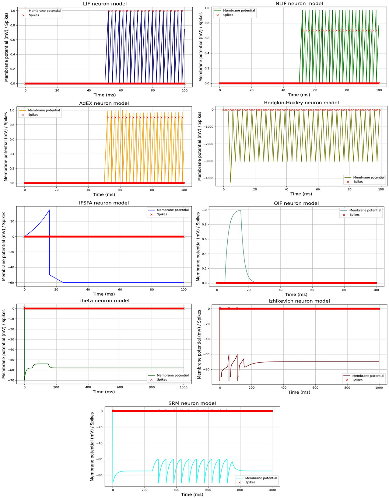
Figure 2. Spiking activity of different SNN models in response to an input current pulse. Each line or curve represents the membrane potential of a specific neuron model, while the red “x” markers indicate the occurrences of spikes. Each model exhibits unique dynamics, producing distinct patterns of spiking activity.